


Some of you have asked when we’ll return to our discussions of college and university financial analysis. Great question. The answer is “now”. We’ll pick up from “The Course-Cost Trap: Why Averages Don’t Reflect the Cost of Growth” (June 4, 2026), which called for using incremental cost to estimate the program and campus margins to be expected at various points in the future.
But it didn’t address these questions:
“What will happen to our revenues, costs, and margins if current conditions were to continue for the next few years? We know there’s momentum in our system, but we don’t know how to measure its effects. What base case should we use for calculating “what-ifs” (outcomes contingent on alternative actions) in our academic program planning?”
This blog provides some answers. The next one will dive more deeply into the incremental costs. A subsequent Blog will consider academic planning goals and objectives, and how to use algorithms and generative AI to work systematically toward their achievement.
Enrollment Data in the Wild
Projecting enrollments was straightforward when I began working on university finances some 50 years ago. Statistical trends, plus consultations with admissions staff and economic advisors, informed our projection of growth rates for graduate and undergraduate admissions. Applying these to the university’s current data allows enrollments to be projected for the next few years. Adjustments to the outyears incorporated our judgments about future economic and government policy shifts.
We made no effort to predict short-term enrollment fluctuations or differentiate trends in academic program enrollment. Both may spawn “wild” changes—“unknown unknowns” that may blindside planners. Looking only at campuswide enrollments and margins exposes the institution to significant forecast errors. Implicit in this approach are two types of problems:
- Embedded Historical Enrollment Fluctuations. This refers to a dip in freshman intakes that results in diminished sophomore, junior, and senior enrollment FTEs—even if intakes have begun moving upward. Institutions may experience cash-flow and other disruptions when such shortfalls appear without warning.
- Unexpected Program Margin Variation due to interactions between enrollment trends and contribution margins. Enrollment trends across programs cancel each other when calculating campus-level enrollments, but there are no such cancelations for program margins. If the high-margin programs are trending downward and the low-margin programs are trending upward, for example, the campus margin will be significantly smaller than predicted from the campus-level data.
These problems are subtle, but consequential. While a few institutions are working with the concepts described here, the vast majority use what is essentially a late 20th-Century methodology—i.e., program-level enrollments “run wild” beneath a relatively smooth (if sometimes alarming) set of campuswide enrollment projections.
Taming the Enrollment Dynamics
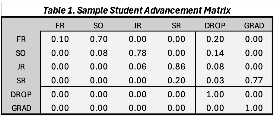
How can we tame the wilderness of program-level enrollment variation? The answer may be familiar to readers of this blog series: we build a program-level model. Table 1 presents a simple example for a particular undergraduate major. (The figures are to facilitate discussion; they do not reflect any particular program or institution.) The table is arranged so its rows show the current year and its columns show the following year, for which predictions are to be made.
The first four rows and columns represent undergraduate cohorts (Freshman, Sophomore, Junior, and Senior), the fifth is Dropouts (students who leave the university early), and the sixth is Graduations (students who receive their degrees). The cohort-to-cohort figures are called transition probabilities: the likelihood that students in a given row this year will end up in one or another of the columns next year. For example, a student in this year’s freshman class would have a 10% probability of repeating freshman year, a 60% probability of moving to sophomore year, a 30% probability of dropping out, and a zero probability of graduating. Notice that the row probabilities sum to 100% (the student must do something).
This is called a “Markov chain model with absorbing states.” Markov is the name of the statistician who first formulated this kind of system. Absorbing states are those which, once entered, can never be exited. Dropout and Graduation are absorbing states. The model may be expanded to include internal and external transfer students. Similar models can be constructed for programs of any length. They can be applied to the campus as a whole, portions of it, individual student majors (programs), or even particular student segments within majors (e.g., athletes and non-athletes).
These Markov student advancement models provide useful information about student flows. They can project forward, year by year, and out to the steady state. Also calculated are the expected fraction of students in each cohort at the steady state, and various other statistics. For example, based on Table 1, the average graduation rate for freshmen is 58% and the average years to graduation is 4.5 years.
The challenge, of course, is to estimate the transition probabilities. The most straightforward approach calculates empirical relative frequencies from institutional databases over a period of years (e.g., 70% of the freshman classes became sophomores, 10% repeated as freshmen, and 20% dropped out). Internet or AI searches will unearth references that describe more powerful estimators. However, even these require larger samples than usually are available at the program level.
Working with small samples presents daunting problems, but combining one’s judgment with the data that are available provides a way forward. The transition probability matrices for our models are small (usually 6 x 6 or smaller) and have many zeros. The probabilities themselves are bounded (each must lie between zero and one and the row sums must equal one). There may be partial evidence, such as reports that freshman dropouts are high or the odds of repeating an academic year are low. Statistics on similar programs or aggregates of programs also may be available. Connect these dots with heuristics (rules of thumb) where applicable, but seriously consider filling the gaps with informed judgment when necessary to describe important phenomena.
Early in my career as a professor and consultant, a senior colleague repeatedly emphasized that, to be useful, decision support models (as we have here) must be complete on important issues. “Robust statistical theory is great, but don’t let its absence deter the creation of a complete model, ”he would say. “Your job as an applied decision scientist is to build models for solving problems that need solving. Use the best tools possible, but waiting for methodological purity is not an option.
Enrollment Dynamics and “What-if” Analysis
The idea behind “what-ifs,” formally known as “contingency analyses,” is to evaluate alternative planning assumptions. This requires estimates of critical cause-effect relations and a starting point or base case. The problems of “embedded historical enrollment fluctuations” and “unexpected program margin variation” confound the base case calculation. Good cause-effect estimates will produce bad predictions when your starting point is unknown. Put another way, your what-if analyses should correct for the embedded enrollment fluctuations and program margin variation. A Markov student advancement model will help you do so.
There are two methods. Apply them at the program level if possible.
- If you’re predicting one year ahead, simply execute the model for one year; if two years, then execute it for two years successively; and so on. The result is an estimate that depends on your current data and whatever intake trend exists for the program.
- If you’re predicting for the indefinite future, calculate the model’s steady state based on the current student intake level. This gives the cohort enrollments to be expected over the long term if current intakes repeat indefinitely; it does not depend on current trends or enrollments.
These calculations are easy when using Excel’s matrix commands. You may consult a chatbot or textbook on Markov models for details.
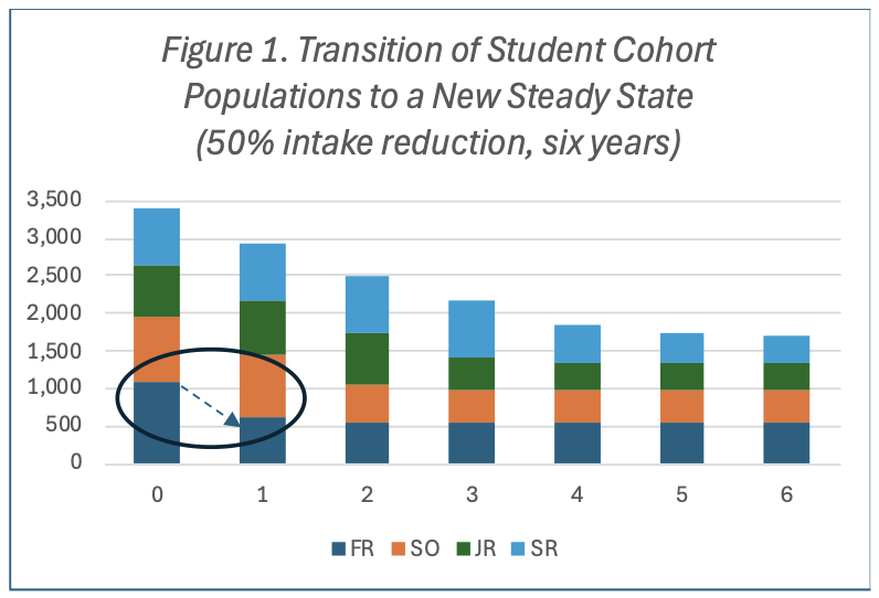
Figure 1 illustrates how one steady state shifts to another when freshman intakes decline, based on the student advancement probabilities in Table 1. (The “initial steady state” assumption states there is no input trend.) FTEs drop from 1,000 in Year 0 (base year) to 500 in Year 1, as shown at the lower left of the diagram. (The amount of change is exaggerated to make the changes more visible.) Convergence is nearly complete in four years, but with a small two-year tail due to the chance of repeating a year.
Switching to real-world numbers, steady-state calculations for an institution with base-year enrollment of about 25 thousand student FTEs spread across some 80 programs showed a 17% enrollment reduction and a 12% margin reduction. This was coupled with a 30% average reduction in faculty teaching loads due to the smaller number of class sections needed to serve the lowered student counts. In other words, the sum of program-by-program enrollment estimates is the same as the campus-wide estimate, but the sum of the program margins may under- or over-estimate the campus margin. These errors may be large enough to warrant planners’ attention.